
Neural Surface Reconstruction using Neuralangelo
Understanding modern neural graphics techniques for extracting 3D surfaces from images

Nvidia recently published a new method for converting photographs to a 3D model with state of the art results. They published the paper in CVPR 2023 in June and just a few weeks ago they published the source code on Github. They provide Neuralangelo as a tool to convert your video captures to meshes and textures (see their Colab notebook here). It already has a great project page that does a good job explaining the method. In this post, I want to take a broader look at the field and the paper to understand how a modern method like Neuralangelo achieves these impressive results.
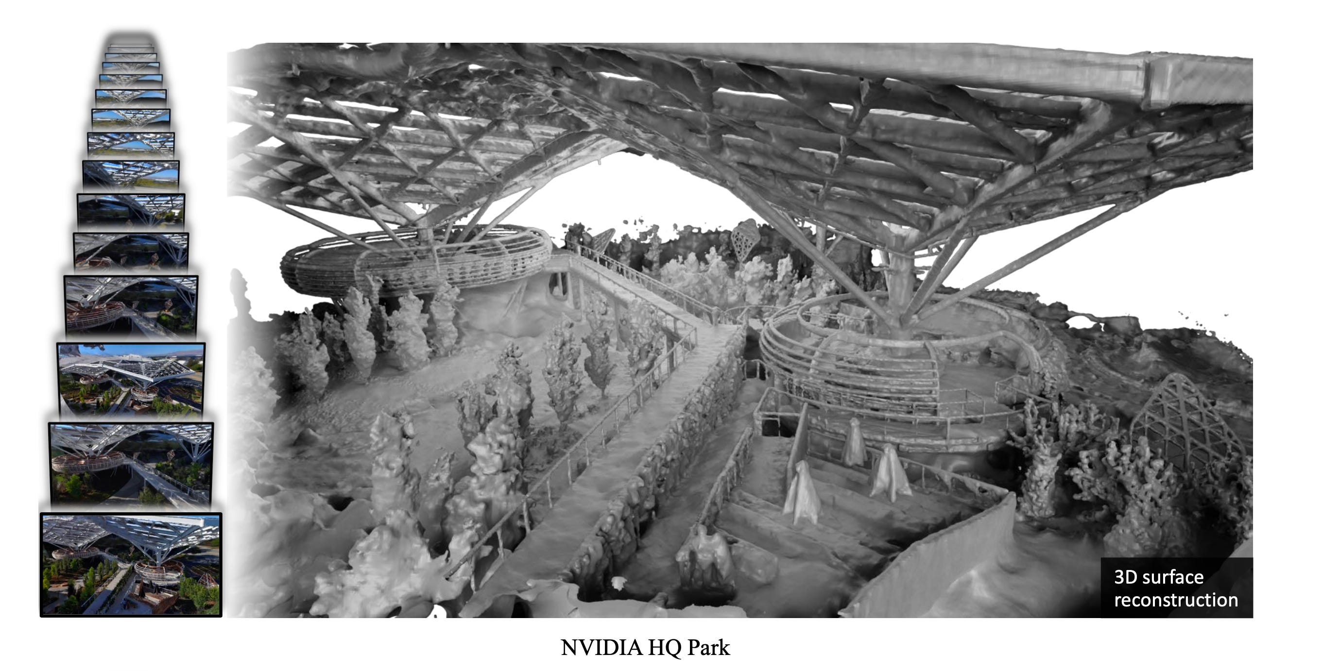
Reconstructing 3D surfaces from multiple images is a classical problem in Computer Vision with a long history. A recently popular approach to this problem is the Neural Graphics approach, where the learning abilities of neural networks are used to represent the 3D scene.
Basically, the input data for the system consists of multiple images of the scene: the photographs or frames from a video sequence capturing the scene from different angles. How many different viewpoints do we need? In the paper they used around 50 images for the DTU Dataset or 263 to 1107 images for the Tanks and Temples dataset.
We may call each pixel of these images an observation of the scene. We want to find a representation of the underlying 3D scene that is consistent with our pixel observations. But how can we come up with such a 3D scene representation? This is the part where the neural networks kick in.
Neural 3D Representations
In classical 3D computer graphics, we represent scenes in terms of surfaces or shapes. To define surfaces, we can use meshes, point clouds or even voxels. We define points in 3D space called vertices, edges between these vertices and triangles or polygons from edges and vertices. These are called explicit 3D representations. GPUs are specialized hardware that processes such data types very efficiently in parallel.
Another type of 3D representation is implicit representations, where we define the surface indirectly. Signed Distance Functions (SDFs) and Occupancy Maps are two examples of this type. An SDF is a function over 3D space where the zero-level set defines the surface. For a point in space, non-zero values of the function determine the distance to the surface and the sign determines which side of the surface our point is on.
We can indeed use triangles and meshes (explicit representations) in a neural rendering setting. Another work from Nvidia, called nvdiffrec, does that by bridging the gap between meshes and SDFs using a differentiable pipeline.
In Neuralangelo, however, we use SDFs directly. Such implicit representations are better suited to be represented by neural network models.
Basics: Neural Radiance Fields
One groundbreaking paper using this approach is the NERF paper from 2020. This paper can be seen as the grandfather of Neuralangelo.
The idea of NERF is simple yet elegant. They optimize an MLP (Multi-Layer Perceptron) to represent a static scene. For a 3D query point and a viewing angle, the network outputs a color and density. Hence, the name Radiance Field.
We can render the scene from any new camera angle by shooting rays from the camera into the scene and sampling the MLP at points along the ray. These samples are then blended to produce the final pixel color. This rendering technique is known as Volume Rendering.
Note that the input of the MLP also includes the view angle. This allows for view-dependent effects, such as reflections, enhancing the realism of the rendered views.
NERFs can create outstanding results, and many papers have since improved on this main idea.
However, there are two main problems with this initial method:
It’s too slow. At least 12 hours of high performance GPU time is needed for optimizing a NERF for a single scene.
NERFs are good for view interpolation (ie. rendering the scene from an unseen camera view). But we may want to extract a traditional mesh representation from the scene. This is non-trivial and requires a separate algorithm.
Instant Neural Graphics Primitives
Among the many variations of the original NERF paper, Nvidia’s Instant Neural Graphics Primitives (InstantNGP; Siggraph 2022) stands out. This is one of the papers that address the speed problem of classical NERFs. Neuralangelo can be viewed as the successor of InstantNGP, with a few modifications.
So what is InstantNGP?
As the name implies, it’s a faster NERF1. This paper uses a combination of two tricks to make the algorithm faster.
Multiresolution Hash Encoding
Faster GPU implementation using fully-fused CUDA kernels
The former allows them to use smaller MLPs. A Smaller network means a smaller number of arithmetic operations, and it reduces the compute time and memory for each MLP. Then they use “fully-fused MLP” implementation from their tiny-cuda-nn library. This gives an additional 10x speedup compared to a naive Python implementation.
The relevant part for our purpose of understanding Neuralangelo is the Multiresolution Hash Encoding part. Let’s have a closer look.
Multiresolution Hash Encoding
Remember when I say the input of the MLP is 3D coordinates and viewing angle? In practice, we don’t give these coordinates and angle values directly to the network. The intuition here is that the coordinates don’t vary too much across the space. Two neighboring points in 3D space have nearly the same coordinate value. This makes it harder for the neural network to discriminate between different points in space. So we convert the 5D input coordinates to another representation. This process is called encoding. The original Nerf paper uses a positional encoding scheme they adopted from the Transformer architecture. They use sin and cosine of the coordinates in different frequency scales.
InstantNGP uses a more advanced parametric encoding scheme where the encoding itself is learned by a neural network.
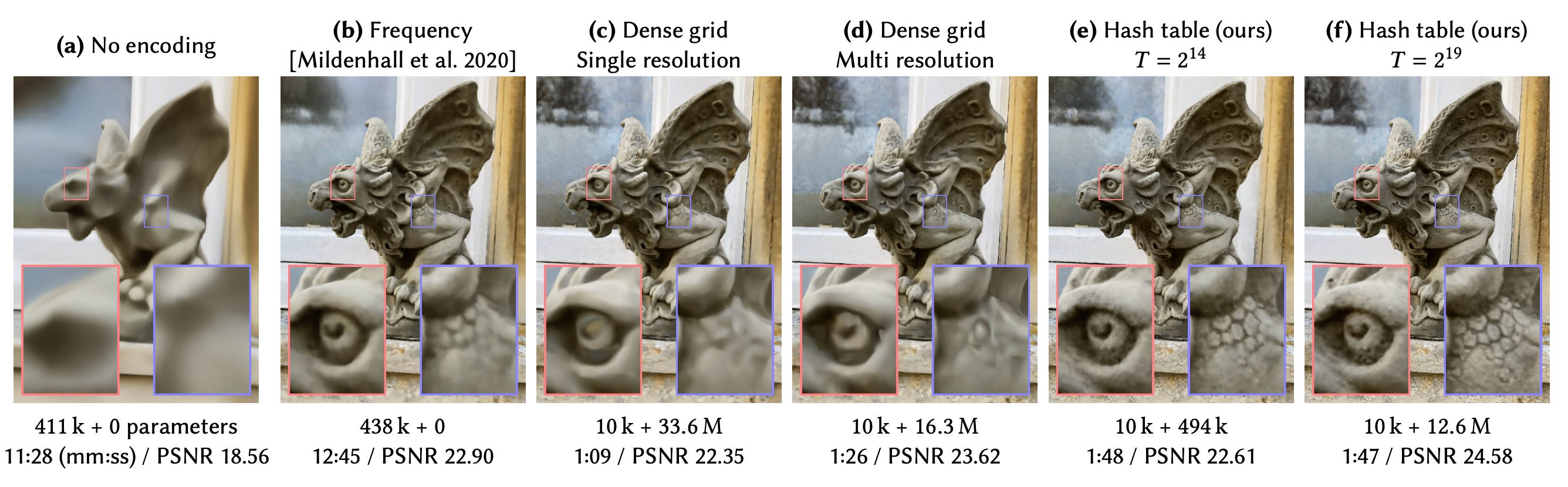
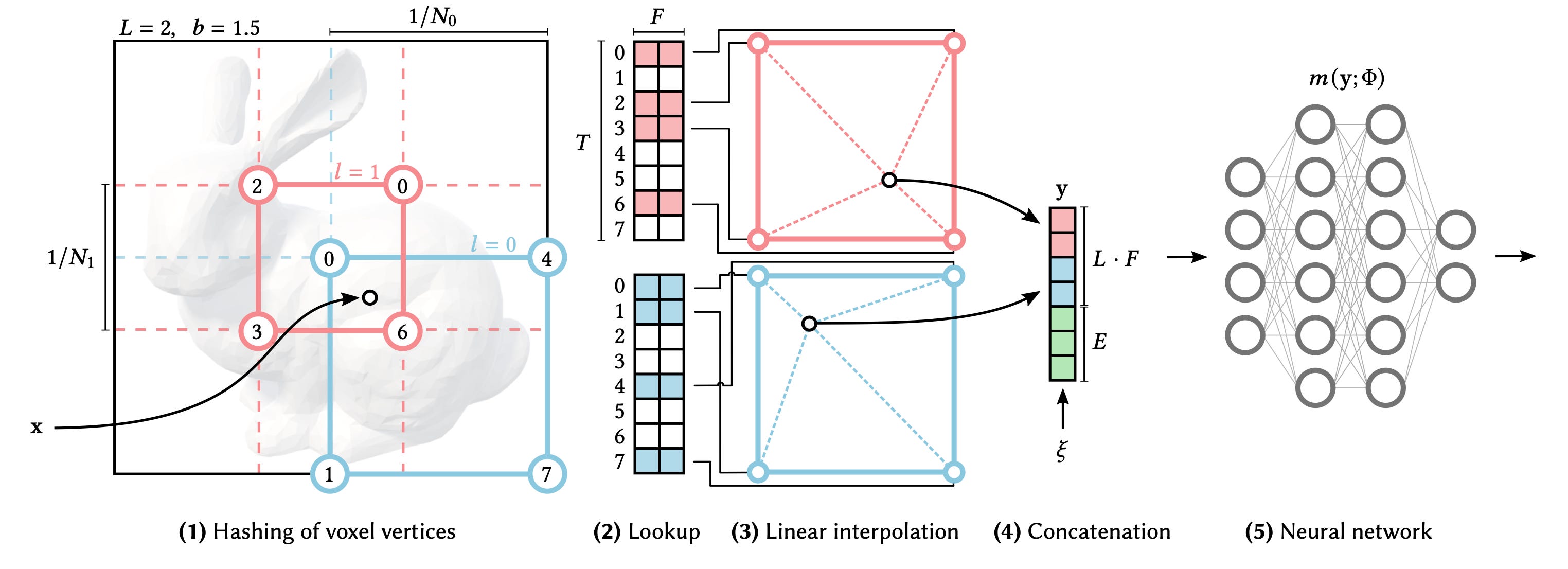
Here is the crux of the method for the curious. Figure below illustrates this in 2D. Imagine there is a 3D voxel grid in the 3D space. For a given 3D point in space, we find the 8 corner points of its enclosing voxel. Each of these 8 points is mapped to an integer value using a known spatial hash function. We use these integers to find the corresponding feature vectors in a lookup table. So each of the 8 points has a feature vector. For our point, we use trilinear interpolation to combine these 8 points to a single feature vector F. This, so far, is the hash encoding part. We want to do this for multiple resolutions. Let L be the number of different resolution levels. Each level has a different grid resolution. We simply concatenate feature vectors from different levels to produce a single feature vector of size L.F.
Back To Neuralangelo
Neuralangelo addresses the 3D Surface Reconstruction problem. People can use multi-view stereo algorithms to solve this problem. Real-world input data is often ambiguous, noisy, and inconsistent. It's challenging for the classical stereo methods to robustly handle these imperfections.
Neural networks have an advantage at this point.
As previously mentioned, Neuralangelo is a successor of InstantNGP. InstantNGP supports various neural graphics primitives, including NERFs and SDFs.
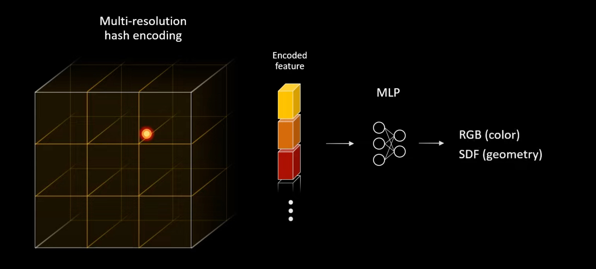
Neuralangelo uses SDF for surface representation. It uses two MLPs: one for color and one for geometry (SDF).
It basically introduces two contributions over InstantNGP:
Higher order derivatives with Numerical Gradients
Coarse-to-fine Optimization scheme
That's basically it. With these two additions, they significantly improve the quality and detail of the reconstructions.
Why choose SDF over density fields? Because we aim to extract the surfaces, and SDF is a more natural representation for this purpose. It models the distance from the surface. Using standard algorithms like Marching Cubes (as in this paper) or Marching Tetrahedra, we can then convert the SDF to triangle meshes.
Now, let's explore these two contributions:
1. Higher Order Derivatives with Numerical Gradients
Here is a useful property of SDF: Its gradient has a magnitude of 1.
Why? The SDF represents distance to the closest surface, and its gradient is simply a unit vector perpendicular to the nearest surface. The SDF changes constantly with respect to distance. Its gradient is essentially the surface normal.
Mathematically, the equation above is called an Eikonal Equation. We want our estimated SDF to behave accordingly. We impose this property of the SDF as an additional regularization to our SDF optimization. We call this term Eikonal Loss:
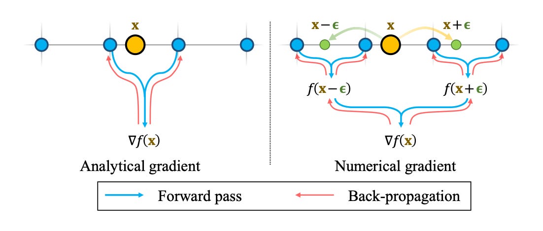
How do we compute this gradient2 (or Surface Normal) ∇f(x) with respect to x? Typically our deep learning framework (they use Pytorch) could handle such gradients. We refer to this as an Analytical Gradient in this context.
The problem is that these Analytical Gradients aren’t continuous across our grid borders.
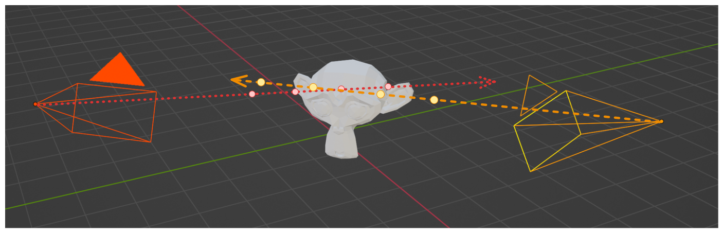
An alternative is to use Numerical Gradients, where we simply sample two points around x along each axis and divide by the step size between these two samples (See the figure below). Since there are 3 axes, we need 6 sample points to compute the gradient at x.
2. Coarse-to-fine Optimization
This is also a popular trick in computer vision tasks. When estimating some property, we first work at a coarser level (i.e., lower resolution) and progressively introduce the finer details. In Neuralangelo, they optimized two parameters in coarse-to-fine manner:
Step Size: This is a hyperparameter we choose when computing the numerical gradient. It’s the distance between the two samples around x. Larger values of the step size have a smoothing effect on the reconstructed surface. This is beneficial for large and continuous surfaces. Smaller values of the step size, on the other hand, are better for reconstructing smaller details. So, they start with a large (coarse) value of step size equal to the coarsest hash grid size and gradually decrease it to the finer grid sizes during optimization.
Hash Grid Resolution: This one is connected to the previous one, the step size. When optimization is working at coarse grid sizes, finer hash grids don’t need to learn anything. So, at the beginning, we only activate the coarse grids and progressively enable finer hash grids when the step size is decreased to that size.
Final Loss Formulation
That’s almost it. One final loss term is used for the mean curvature to impose further smoothness on the surface. They approximate this using a discrete Laplacian.
And the final loss is:
with corresponding weights as hyperparameters.
Final Thoughts
The field of neural graphics is progressing at a remarkable speed. In this article, we have covered the basic ideas behind state-of-the-art methods such as NERFs, InstantNGP, and Neuralangelo. These papers have emerged in the last 2-3 years and they already deliver impressive results. I hope this article helps you understand the foundational concepts behind these achievements.
In fact, the paper covers multiple Neural Graphics Primitives. Radiance Fileds, Signed Distance Fields and Gigapixel Images (where MLP learns converting given 2D coordinates to RGB values). All these primitives are basically MLPs with different input and output meanings.
When they say Higher Order Derivatives they mean this surface normal ∇f(x) and the Laplacian of f(x).